2025-05-30 - Dev Log 2
Tldr
Good stuff here, I just hadn’t really thought about the fact that a lot of the columns I was including in my model here were leaking future information and making the model useless for predictions.
Starting over with different source data
I decided this table might be a little better for this task
SELECT period_start, period_end, duration, u_diff, d_diff, t_diff, u_rate, d_rate, t_rate
FROM "SECV_SCRAPE".scrape_data_intervals
WHERE duration > interval '0 seconds'  -- filter out zero or negative durations if any
	AND u_diff >= 0 AND d_diff >= 0 AND t_diff >= 0
	AND u_rate >= 0 AND d_rate >= 0 AND t_rate >= 0
	and d_rate <= 125000000
ORDER BY period_end desc;
Which looks like this:
| period_start | period_end | duration | u_diff | d_diff | t_diff | u_rate | d_rate | t_rate |
|---|---|---|---|---|---|---|---|---|
| 5/30/25 17:00 | 5/30/25 18:00 | 01:00:00 | 676,281,904 | 3,007,805,433 | 3,684,087,337 | 187,842 | 835,437 | 1,023,278 |
| 5/30/25 16:00 | 5/30/25 17:00 | 01:00:00 | 665,539,331 | 2,792,166,428 | 3,457,705,759 | 184,863 | 775,563 | 960,426 |
| 5/30/25 15:00 | 5/30/25 16:00 | 01:00:00 | 1,413,274,412 | 28,387,410,765 | 29,800,685,177 | 392,526 | 7,884,385 | 8,276,911 |
| 5/30/25 14:00 | 5/30/25 15:00 | 01:00:00 | 3,112,186,339 | 27,515,570,457 | 30,627,756,796 | 864,592 | 7,644,064 | 8,508,656 |
| 5/30/25 13:00 | 5/30/25 14:00 | 00:59:59 | 1,804,309,482 | 6,606,510,477 | 8,410,819,959 | 501,305 | 1,835,536 | 2,336,841 |
Just applying the most basic cleanup right in the query (e.g. no negative values) there did appear to be some cleanup that needed to be done…
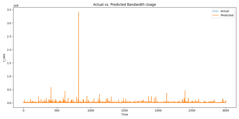
So I then added and d_rate <= 125000000 which is the theoretical maximum downstream transfer rate. Which helped a bit:
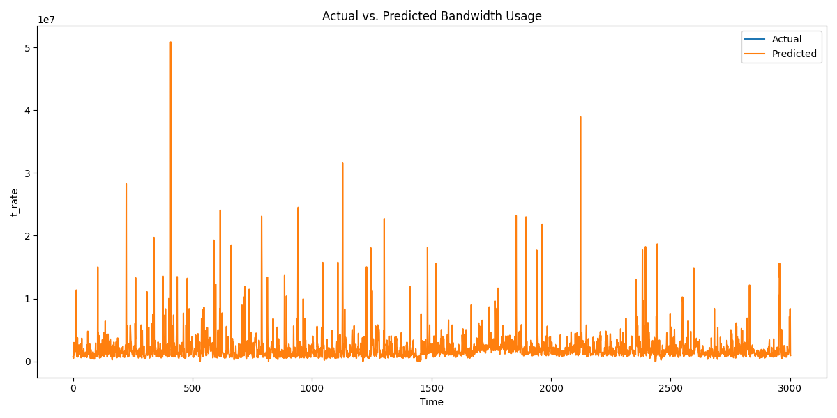
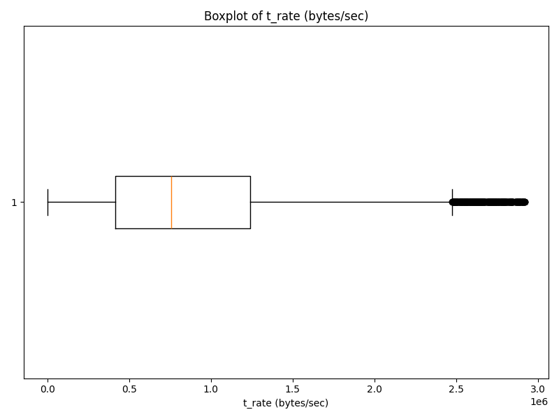
But that’s still pretty bad so I generated a box plot too just to get an idea of what was going on:
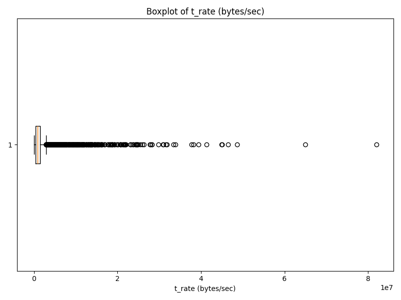 That paints a pretty clear picture doesn’t it? So, arming myself with the power of basic statistics I applied the following filtering to the df at the end of the ETL step:
    Q1 = df['t_rate'].quantile(0.25)
    Q3 = df['t_rate'].quantile(0.75)
    IQR = Q3 - Q1
    upper_bound = Q3 + 1.5 * IQR

    # Filter out outliers
    df_filtered = df[df['t_rate'] <= upper_bound]
    print(f"Rows before: {len(df)}, after filtering: {len(df_filtered)}")
and lo, the data was calmed, to some extent:
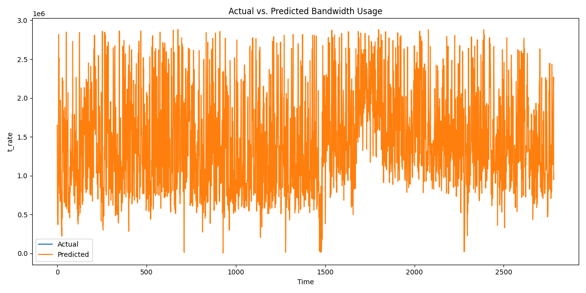
Check out these error values too:
[model_training_and_evaluation] Mean Absolute Error (MAE): 21279.986311886292
[model_training_and_evaluation] Root Mean Squared Error (RMSE): 30238.041370875548
21kb and 30kb respectively, and the RMS value is quite close to the mean value now indicating that the worst of the outliers have been culled.
Hyperparameter Tuning
Wow this is cool
Quick dictionary definition for context: Hyperparameters are settings that you, the data scientist, set before training begins. They are not learned from the data. Instead, they control how the learning process itself works.
I implemented a randomized search and this improved the models accuracy by a lot
[model_training_and_evaluation] Mean Absolute Error (MAE): 10837.451371471327
[model_training_and_evaluation] Root Mean Squared Error (RMSE): 19982.03328426008
The RMSE value is now better than the previous MAE value
# 1. Prepare the Data
    # Define Features and Target
    features = [col for col in df.columns if col not in [target_col, "period_start", "period_end"]]
    target = target_col

    # Split Data into Training and Testing Sets (Time-Series-Aware)
    X = df[features]
    y = df[target]
    X_train, X_test, y_train, y_test = train_test_split(X, y, test_size=test_size, shuffle=False)

    # Scale Features
    scaler = StandardScaler()
    X_train = scaler.fit_transform(X_train)
    X_test = scaler.transform(X_test)

    # Define your parameter search space
    param_dist = {
        'n_estimators': [100, 200, 300, 400, 500],
        'max_depth': [3, 5, 7, 10, 12, 15],
        'learning_rate': [0.005, 0.01, 0.025, 0.05, 0.1, 0.2, 0.3],
        'subsample': [0.5, 0.6, 0.7, 0.8, 0.9, 1.0],
        'colsample_bytree': [0.5, 0.6, 0.7, 0.8, 0.9, 1.0],
        'reg_alpha': [0, 0.01, 0.05, 0.1, 0.5, 1, 2, 5, 10],
        'reg_lambda': [0.5, 1, 1.5, 2, 5, 10, 20],
        'min_child_weight': [1, 2, 3, 5, 7, 10],
        'gamma': [0, 0.01, 0.1, 0.2, 0.5, 1, 2, 5]
    }

    # Initialize the model
    model = xgb.XGBRegressor(objective='reg:squarederror', random_state=42)

    # Set up the randomized search
    search = RandomizedSearchCV(
        estimator=model,
        param_distributions=param_dist,
        n_iter=100,  # Number of parameter settings sampled
        scoring='neg_mean_absolute_error',  # Use MAE for scoring
        cv=3,  # 3-fold cross-validation
        verbose=2,
        n_jobs=-1  # Use all available cores
    )

    # Fit the search to your training data
    search.fit(X_train, y_train)

    # Print the best parameters and score
    print("Best hyperparameters:", search.best_params_)
    print("Best MAE (CV):", -search.best_score_)

    # Use the best estimator for predictions
    best_model = search.best_estimator_
    y_pred = best_model.predict(X_test)

    # 3. Train the Model
    best_model.fit(X_train, y_train)
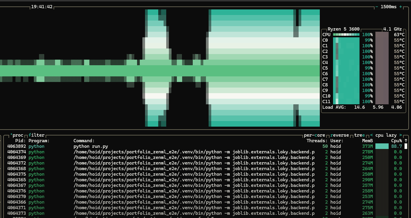
This is the first thing I’ve noticed that really chews up some CPU cycles:
Added some code to display which features have the greatest effect on the model:
[model_training_and_evaluation] Feature importance (gain):
[model_training_and_evaluation] d_rate: 669,571,940,352
[model_training_and_evaluation] u_rate: 591,558,737,920
[model_training_and_evaluation] t_diff:  68,015,915,008
[model_training_and_evaluation] duration: 2,225,079,296
[model_training_and_evaluation] year:       333,116,640
[model_training_and_evaluation] d_diff:     105,182,528
[model_training_and_evaluation] u_diff:      48,728,988
[model_training_and_evaluation] month:       42,900,036
[model_training_and_evaluation] day_of_year: 34,279,040
[model_training_and_evaluation] day_of_week: 28,938,516
[model_training_and_evaluation] hour:        28,094,210
The only one here that was kind of surprising to me was that year was pretty high on the list. Then again back in 2015 when I started logging this data my monthly cap was only 400GB. The cap was raised and eventually removed altogether over time, so it does make sense that there would be a correlation there. I think as time goes on and the model is retrained year will drop towards the bottom of the list.
All that being said I think it’s important to point how how much more important the download rate and upload rate are than the rest. It’s pretty obvious from the listing above but here’s a crappy matplotlib plot to really hammer it home:
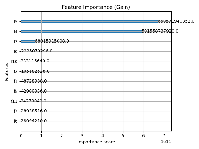 Logically, it makes sense that download rate would end up carrying a little more weight since my download speed (
1000mbps) is much higher than my upload speed (100mbps).
It didn’t score that much higher though; perhaps that’s because I do have a lot of upstream traffic, albeit at a lower speed, I am almost constantly uploading data.
 Despite the upload speed being 10x lower than download on average for the last 10 years, the downstream total is only 24% higher.
Ensemble Models
Why not right? I trained a Random Forest model and that is actually getting better numbers than the XGBoost has so far. These libraries make it so simple to do crazy things like training an ensemble model to effectively use predictions from both of these models. I wonder if it will be any good…
    # Prepare meta-learner training data (predictions of base models on training set)
    meta_X_train = np.column_stack((
        best_xgb_model.predict(X_train),
        best_rf_model.predict(X_train)
    ))
    meta_X_test = np.column_stack((
        best_xgb_model.predict(X_test),
        best_rf_model.predict(X_test)
    ))

    # Train meta-learner
    meta_model = LinearRegression()
    meta_model.fit(meta_X_train, y_train)

    # Predict with meta-learner
    y_pred_ensemble = meta_model.predict(meta_X_test)

    # Evaluate stacking ensemble
    mae_ensemble = mean_absolute_error(y_test, y_pred_ensemble)
    rmse_ensemble = np.sqrt(mean_squared_error(y_test, y_pred_ensemble))

    print(f"Stacking Ensemble Mean Absolute Error (MAE): {mae_ensemble}")
    print(f"Stacking Ensemble Root Mean Squared Error (RMSE): {rmse_ensemble}")
lol… nope
XGBoost Mean Absolute Error (MAE):                12,060
XGBoost Root Mean Squared Error (RMSE):           23,070

Random Forest Mean Absolute Error (MAE):           8,605
Random Forest Root Mean Squared Error (RMSE):     15,756

Stacking Ensemble Mean Absolute Error (MAE):      12,970
Stacking Ensemble Root Mean Squared Error (RMSE): 24,815
Both of the methods I’ve tried in order to ensemble these together have just come out worse than both inputs. I’ll have to dig into this more though, super interesting.
Time Series Cross Validation
I did this last time in a separate step just as a validation check, but apparently you can just build it into the Hyperparameter Tuning
Note the tscv object now being incorporated into the RandomizedSearchCV call:
	print("Performing Time Series Cross-Validation for Random Forest...")
    tscv = TimeSeriesSplit(n_splits=5)  # You can adjust the number of splits

    param_dist_rf = {
        'n_estimators': [100, 200, 300, 400, 500, 600],
        'max_depth': [None, 5, 10, 15, 20, 25, 30],
        'min_samples_split': [2, 5, 10, 15, 20],
        'min_samples_leaf': [1, 2, 4, 6, 8],
        'max_features': ['sqrt', 'log2', 0.5, 0.7, 1.0],  # Removed 'auto'
        'bootstrap': [True, False]
    }

    rf_model = RandomForestRegressor(random_state=42)

    search_rf = RandomizedSearchCV(
        estimator=rf_model,
        param_distributions=param_dist_rf,
        n_iter=50,  # Adjust as needed
        scoring='neg_mean_absolute_error',
        cv=tscv,
        verbose=2,
        n_jobs=-1
    )

    search_rf.fit(X_train, y_train)
This provided the best results yet:
Random Forest Mean Absolute Error (MAE):       6,818
Random Forest Root Mean Squared Error (RMSE): 14,056

Random Forest Feature Importance:
u_rate: 0.42156569915756137
d_rate: 0.41094150337087687
t_diff: 0.12404854944557978
d_diff: 0.017410409186994484
duration: 0.011682057274900846
u_diff: 0.007608643644552923
year: 0.006277061690141597
day_of_year: 0.00023217906996870002
hour: 0.00011289598208008557
month: 5.3290942979228746e-05
day_of_week: 3.845530834859385e-05
quarter: 2.006413364359434e-05
is_weekend: 9.19079237169601e-06
I think I have a pretty well preforming model, an average error of ~7KB/sec when my typical daily average rate is something like 2,109KB/sec seems solid.